Honors Capstone Data Exploration

Data Description

My Honors Capstone data on the distribution and diversity of macrophytes (aquatic plants) in the Carmel River Watershed will be used for this project. I collected this data from the spring of 2025 until the end of fall 2025. I also joined additional variables from the EPA’s StreamCat dataset (Hill et al. 2016) which are variable means for each smaller watershed in the Carmel River Watershed area. If you would like to know more about my findings, please check out my Final Honors Capstone Slides.

• My collected data has 279 rows and 28 variables, 11 character variables, 15 double variables, and 2 time variables.

• Methods for Data Collection and variables collected:

  • Do a 50 m transect on both sides of the river, 1 meter out from shore, recorded plants every time seen, within 1 meters of each side of the tape (overall 4 meters recorded)

  • When a stream is less than or equal to 2 meters wide, I only surveyed one transect in the middle of the river, to cover the full two meters.

  • Every time a plant was found I measured:

    • Depth (m)

    • Velocity (m/s)

    • Substrate size (mm)

    • Plant name and number of individuals or range/cover area on the transect

  • Measure at each transect overall:

    • Canopy cover facing north, south, east, and west, [these numbers were averaged, then multiplied by 4 and divided by product of 17*4 (freshwater ecology standard)]

    • Percentage of the 50-meter transects that were riffle, pool, run, or glide.

    • Water temperature (°C)

    • pH

    • Conductivity(ms/cm)

    • TDS (g/L)

    • Dissolved oxygen [DO] (mg/L) and Dissolved oxygen (%)

    • Salinity (parts per thousand)

• Downloaded StreamCat Variables:

  • Mean runoff (mm)

  • Mean elevation (m)

  • Watershed area (km2)

  • Percent base stream flow index

  • Mean annual precipitation from 1991-2020 (mm)

  • Mean annual temperature from 1991-2020 (C°)

  • Mean percent lithological calcium oxide (CaO) content

• Research Questions and Hypotheses for Overall Project:

  • What aquatic plant species are present in the Carmel River Watershed and what species are the most abundant?
    • H: Non-natives more abundant.
  • Which environmental factors affect the distribution and diversity of aquatic plants in the Carmel River Watershed in Monterey County, CA? 
    • H: Diversity increases with increasing depth, sunlight, water quality, but decreases with increasing flow and substrate size.

• Purpose of this Project Page: To explore and clean my Honors Capstone data before I start modelling the influence of these environmental factors on macrophyte abundance and presence or absence.

Data Cleaning

• Changed the substrate and velocity variables to remove “>” or “<” symbols so that they can be numeric variables. I did this with mutate().
• I dealt with missing data. I removed NA data from the velocity variable and change NA values in the depth variable to zero using mutate().
• Creation of new variables:
  • Stem count variable: called calc_stem_abundance_m2 by multiplying number of individuals by 0.09 (accounting for each individual as 900 cm^2 on average for an estimate)
  • Final Abundance variable: Combining the stem count variable and cover area. I used cover area when the value for the number of individuals is NA or individuals are greater than or equal to 150 (this may be a less accurate estimate of individuals so using cover area is a better estimate in this case). I also added a clause for using the cover area variable instead of individuals for annual grass if individuals are greater than 5 (as it is difficult to count individual blades of grass).
  • Rooted versus floating variable: by combining the values of emergent and submergent into one value of “rooted” and keeping the value of “floating” the same.
  • creating a presence/absence column for each species at each site with 1 indicating presence and 0 indicating absence.
• Variable Summarization:
  • I will grouped my data by species, transect location and site. Then, I took the sum of the final_abundance, and calculated the mean for all my environmental variables, for each of the groupings.
  • Created final datasets for presence-absence and abundance data with these summarizations
• Pivoting:
  • I used pivot_wider to create the initial presence/absence matrix and then pivot_longer to add the environmental variables to the new presence/absence dataset.
• Joining Data:
  • Joined additional environmental variables from the StreamCat dataset to my new abundance and presence/absence datasets.
• Other aspects that needed to be “fixed” in order to make my data visualizations:
  • used the janitor package to clean my variable names and make it easier to fully clean my data.
  • Excluded the variables: location_coordinates, date, observers, start_time, end_time, as they weren’t important for my analysis.
  • DO % as well as the glide variable were removed due to redundancy in other variables as well as limited data.
  • Salinity and TDS were also removed as they are derivative calculations of conductivity which was kept.
  • Mean annual air temperature was removed as well since it doesn’t change much over the years and the field water temperature measurement is a better metric for aquatic plants.

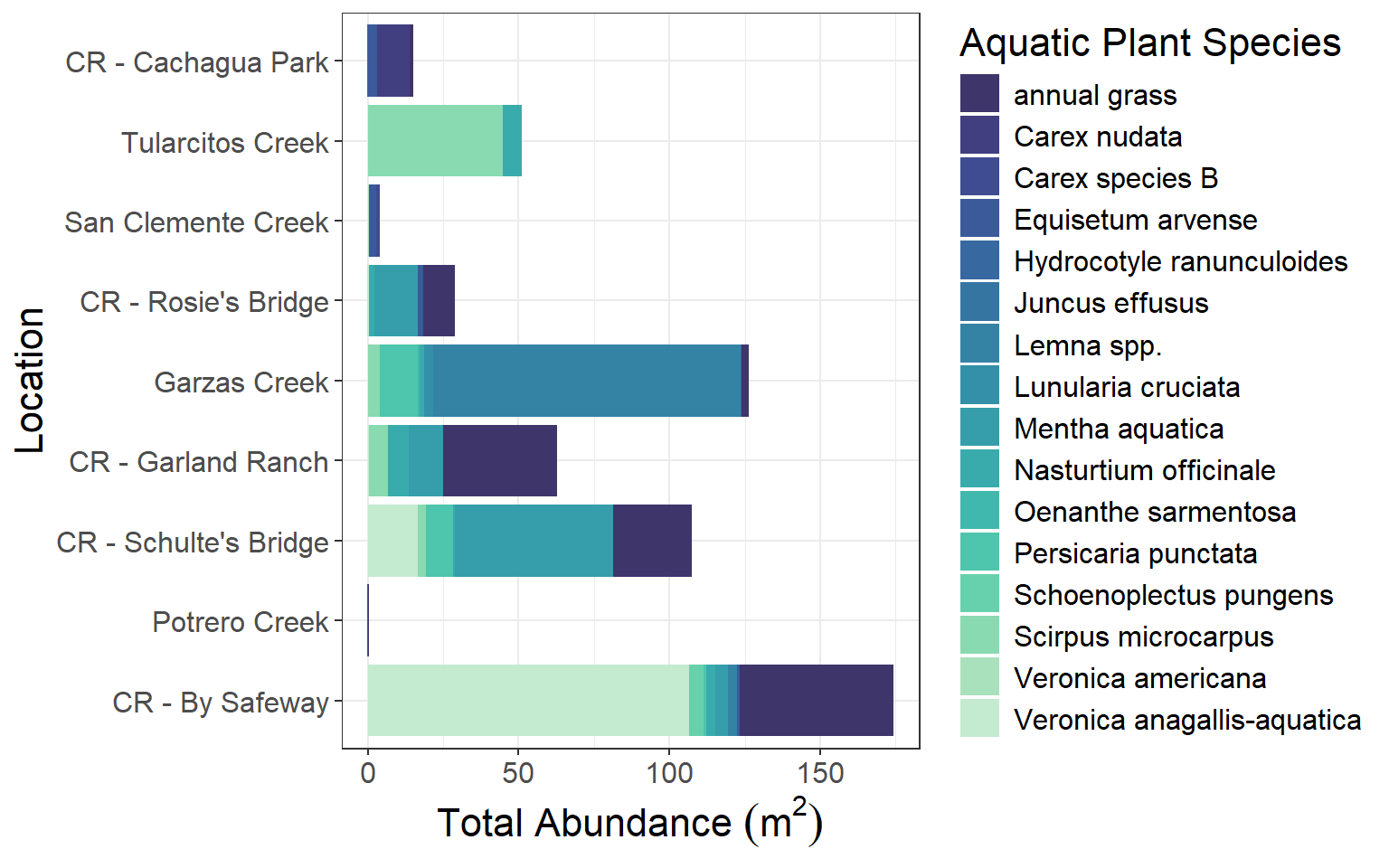
Visualization 1: Abundance of Different Species across Sites

The purpose of the visualization below is to show the change in abundance of my 16 aquatic plant species found throughout my 9 sites as well as overall abundance of aquatic plants throughout my sites. The sites are arranged on the graph from upstream (on the top of the graphic) to downstream on the bottom of the graphic. As you can see below, sites further downstream tend to have higher abundance of aquatic plants, except for my tributary sites which are outliers (my tributary sites are Potrero Creek, Tularcitos Creek, San Clemente Creek, and Garzas Creek). The “Carmel River - By Safeway” site has overall the highest abundance of aquatic plants and is the furthest downstream. The sites further downstream and on the main stem of the Carmel River are in the more urban areas of the Carmel Valley and are larger rivers, which may be contributing to this trend in aquatic plant abundance.

Figure 1. Bar chart showing species abundance at each site. CR stands for Carmel River on the plot. Sites are ordered upstream to downstream.

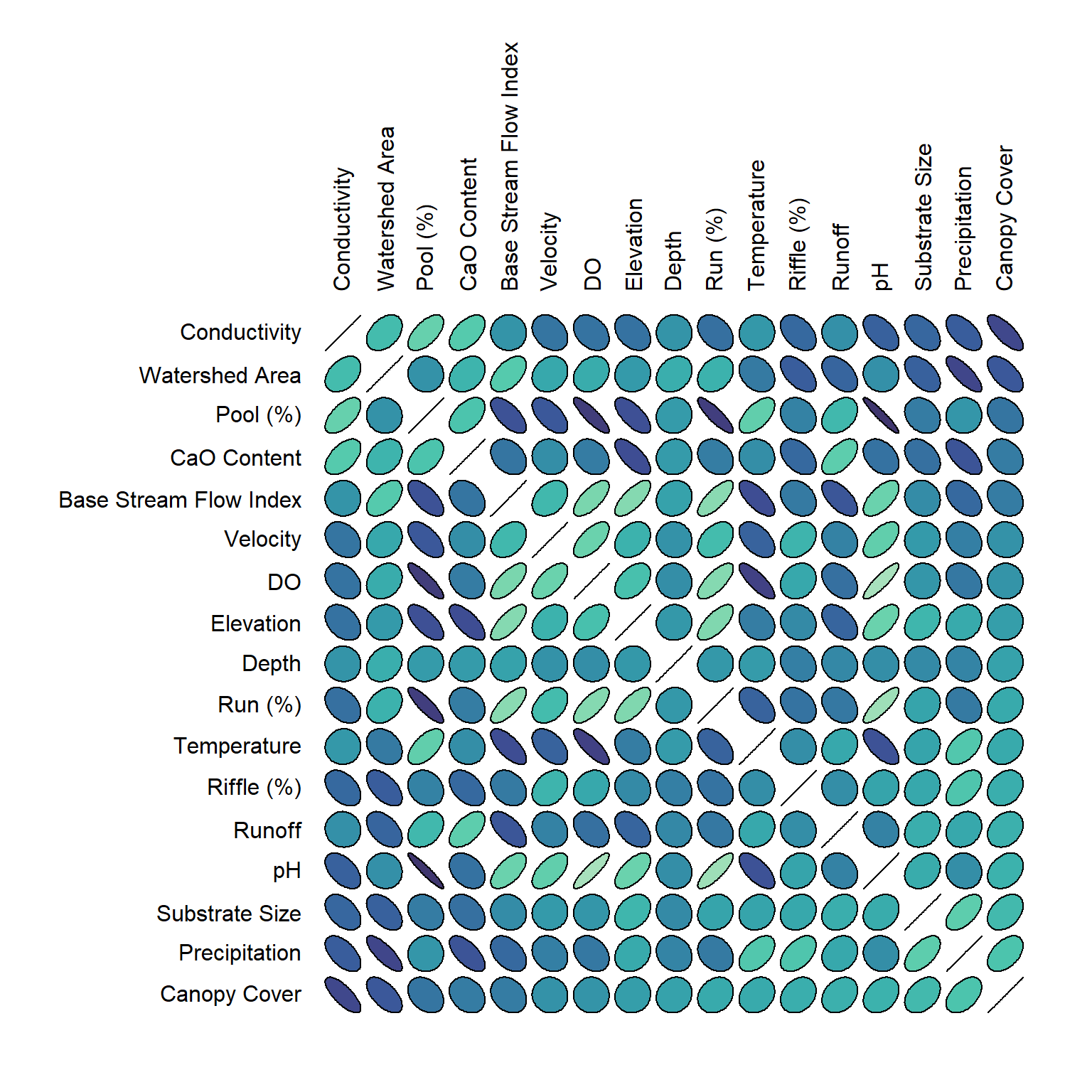
Visualization 2: Correlogram of important variables against each other

The purpose of this second visualization is to understand the relationships between my environmental predictors and determine if there are any strong correlations present. Most relationships appear to be not very strong or have are relatively strong negative relationships. Some of the strongest relationships appear to be pH and pool % (positive) as well as pH and run % (negative). Dissolved oxygen (DO) also appears to be fairly correlated with pH (positive) as well as pool (negative), and run (positive) percentage variables. These correlations make sense as it is well understood that the type of flow can influence dissolved oxygen levels and other aspects of water chemistry. These types of inherent relationships need to be considered with modelling and other statistical analysis to understand the relationships between the environmental predictors and species abundance or presence-absence. (Due to such relationships linear and logistic regression models were abandoned in later analysis since I did not meet the assumptions for these models and I moved on to Random Forest Modelling for my final capstone project).

Figure 2. Correlogram of important environmental predictors to understand strength of collinearity between variables.